Backpropagation in a convolutional layer

Backpropagation in a convolutional layer

Working on the Stanford course CS231n: Convolutional Neural Networks for Visual Recognition. I did not manage to find a complete explanation of how backprop math is working. So here is a post detailing step by step how this key element of Convnet is dealing with backprop.

Introduction

Motivation

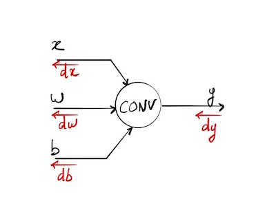
The aim of this post is to detail how gradient backpropagation is working in a convolutional layer of a neural network. Typically the output of this layer will be the input of a chosen activation function (relufor instance). We are making the assumption that we are given the gradient dy backpropagated from this activation function. As I was unable to find on the web a complete, detailed, and “simple” explanation of how it works. I decided to do the maths, trying to understand step by step how it’s working on simple examples before generalizing. Before further reading, you should be familiar with neural networks, and especially forward pass, backpropagation of gradient in a computational graph and basic linear algebra with tensors.

Notations

* will refer to the convolution of 2 tensors in the case of a neural network (an input x and a filter w).

• When xand w are matrices:
• if xand w share the same shape, x*w will be a scalar equal to the sum across the results of the element-wise multiplication between the arrays.
• if wis smaller the x, we will obtain an activation map y where each value is the predefined convolution operation of a sub-region of x with the sizes of w. This sub-region activated by the filter is sliding all across the input array x.
• if xand w have more than 2 dimensions, we are considering the last 3 ones for the convolution, and the last 2 ones for the highlighted sliding area (we just add one depth to our matrix)

Notations and variables are the same as the ones used in the excellent Stanford course on convolutional neural networks for visual recognition and especially the ones of assignment 2. Details on convolutional layer and forward pass will be found in this video and an instance of a naive implementation of the forward pass post.

Goal

Our goal is to find out how gradient is propagating backwards in a convolutional layer. The forward pass is defined like this:

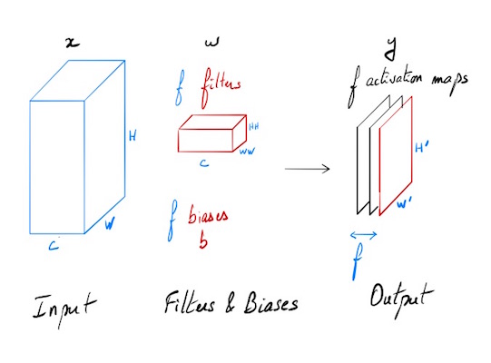
The input consists of N data points, each with C channels, height H and width W. We convolve each input with F different filters, where each filter spans all C channels and has height HH and width WW.

Input:

• x: Input data of shape (N, C, H, W)
• w: Filter weights of shape (F, C, HH, WW)
• b: Biases, of shape (F,)
• conv_param: A dictionary with the following keys:
  • ‘stride’: The number of pixels between adjacent receptive fields in the horizontal and vertical directions.
  • ‘pad’: The number of pixels that will be used to zero-pad the input.

During padding, ‘pad’ zeros should be placed symmetrically (i.e equally on both sides) along the height and width axes of the input.

Returns a tuple of:

• out: Output data, of shape (N, F, H’, W’) where H’ and W’ are given by H’ = 1 + (H + 2 * pad - HH) / stride W’ = 1 + (W + 2 * pad - WW) / stride
• cache: (x, w, b, conv_param)

Forward pass

Generic case (simplified with N=1, C=1, F=1)

N=1 one input, C=1 one channel, F=1 one filter.

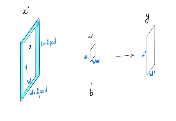
• $x$ : $H \times W$
• $x’ = x$ with padding
• $w$ : $HH \times WW$
• $b$ bias : scalar
• $y$ : $H’\times W’$
• stride $s$

$\forall (i,j) \in [1,H’] \times [1,W’]$

\[y_{ij} = \left (\sum_{k=1}^{HH} \sum_{l=1}^{WW} w_{kl} x'_{si+k-1,sj+l-1} \right ) + b \tag {1}\]

Specific case: stride=1, pad=0, and no bias.

\[y_{ij} = \sum_{k} \sum_{l} w_{kl} \cdot x_{i+k-1,j+l-1} \tag {2}\]

Backpropagation

We know:

$dy = \left(\frac{\partial L}{\partial y_{ij}}\right)$

We want to compute $dx$, $dw$ and $db$, partial derivatives of our cost funcion L. We suppose that the gradient of this function has been backpropagated till y.

Trivial case: input x is a vector (1 dimension)

We are looking for an intuition of how it works on an easy setup and later on we will try to generalize.

Input

\[x = \begin{bmatrix} x_1\\ x_2\\ x_3\\ x_4 \end{bmatrix}\] \[w = \begin{bmatrix} w_1\\ w_2 \end{bmatrix}\] \[b\]

Output

\[y = \begin{bmatrix} y_1\\ y_2\\ y_3 \end{bmatrix}\]

Forward pass - convolution with one filter w, stride = 1, padding = 0

\[y_1 = w_1 x_1 + w_2 x_2 + b\\ y_2 = w_1 x_2 + w_2 x_3 + b \tag{3}\\ y_3 = w_1 x_3 + w_2 x_4 + b\]

Backpropagation

We know the gradient of our cost function L with respect to y:

\[dy = \frac{\partial L}{\partial y}\]

This can be written with the Jacobian notation:

\[\begin{align*} & dy = \begin{bmatrix} \frac{\partial L}{\partial y_1} & \frac{\partial L}{\partial y_2} & \frac{\partial L}{\partial y_3} \end{bmatrix} \\ & dy = \begin{bmatrix} dy_1 & dy_2 & dy_3 \end{bmatrix} \end{align*}\]

dy and y share the same shape:

\[dy = (dy_1 , dy_2 , dy_3)\]

We are looking for

\[dx=\frac{\partial L}{\partial x}, dw=\frac{\partial L}{\partial w}, db=\frac{\partial L}{\partial b}\]

db

\[db=\frac{\partial L}{\partial y}\cdot \frac{\partial y}{\partial b} = dy\cdot\frac{\partial y}{\partial b}\]

Using the chain rule and the forward pass formula (1), we can write:

\[db = \sum_{j}\frac{\partial L}{\partial y_j}\cdot \frac{\partial y_j}{\partial b} = \begin{bmatrix} dy_1 & dy_2 & dy_3 \end{bmatrix} \cdot \begin{bmatrix} 1\\ 1\\ 1 \end{bmatrix}\] \[\Rightarrow db=dy_1+dy_2+dy_3\]

dw

\[dw=\frac{\partial L}{\partial y}\cdot \frac{\partial y}{\partial w} = dy\cdot\frac{\partial y}{\partial w}\] \[\frac{\partial y}{\partial w} = \begin{bmatrix} \frac{\partial y_1}{\partial w_1} & \frac{\partial y_1}{\partial w_2}\\ \frac{\partial y_2}{\partial w_1} & \frac{\partial y_2}{\partial w_2}\\ \frac{\partial y_3}{\partial w_1} & \frac{\partial y_3}{\partial w_2}\\ \end{bmatrix}\] \[\frac{\partial y}{\partial w} = \begin{bmatrix} x_1 & x_2\\ x_2 & x_3\\ x_3 & x_4\\ \end{bmatrix}\] \[\begin{bmatrix} dy_1 & dy_2 & dy_3 \end{bmatrix} \cdot \begin{bmatrix} x_1 & x_2\\ x_2 & x_3\\ x_3 & x_4\\ \end{bmatrix}\] \[dw_1 = x_1 dy_1 + x_2 dy_2 + x_3 dy_3 \\ dw_2 = x_2 dy_1 + x_3 dy_2 + x_4 dy_3\]

We can notice that dw is a convolution of the input x with a filter dy. Let’s see if it’s still valid with a added dimension.

\[dw = \begin{bmatrix} x_1 \\ x_2 \\ x_3 \\ x_4 \end{bmatrix} * \begin{bmatrix} dy_1 \\ dy_2 \\ dy_3 \end{bmatrix}\]

dx

\[dx=\frac{\partial L}{\partial y}\cdot \frac{\partial y}{\partial x} = dy^T\cdot\frac{\partial y}{\partial x}\] \[\frac{\partial y}{\partial x} = \begin{bmatrix} \frac{\partial y_1}{\partial x_1} & \frac{\partial y_1}{\partial x_2} & \frac{\partial y_1}{\partial x_3} & \frac{\partial y_1}{\partial x_4}\\ \frac{\partial y_2}{\partial x_1} & \frac{\partial y_2}{\partial x_2} & \frac{\partial y_2}{\partial x_3} & \frac{\partial y_2}{\partial x_4}\\ \frac{\partial y_3}{\partial x_1} & \frac{\partial y_3}{\partial x_2} & \frac{\partial y_3}{\partial x_3} & \frac{\partial y_3}{\partial x_4}\\ \end{bmatrix}\] \[\frac{\partial y}{\partial x} = \begin{bmatrix} w_1 & w_2 & 0 & 0\\ 0 & w_1 & w_2 & 0\\ 0 & 0 & w_1 & w_2\\ \end{bmatrix}\] \[\begin{align*} &dx_1 = w_1 dy_1\\ &dx_2 = w_2 dy_1 + w_1 dy_2 \\ &dx_3 = w_2 dy_2 + w_1 dy_3 \\ &dx_4 = w_2 dy_3 \end{align*}\]

Once again, we have a convolution. A little bit more complex this time. We should consider an input dy with a 0-padding of size 1 convolved with an “inverted” filter w like $(w_2, w_1)$

\[dx = \begin{bmatrix} 0 \\ dy_1 \\ dy_2 \\ dy_3 \\ 0 \end{bmatrix} * \begin{bmatrix} w_2 \\ w_1 \end{bmatrix}\]

Next step will be to have a look on how it works on small matrices.

Input x is a matrix (2 dimensions)

Input

\[x = \begin{bmatrix} x_{11} &x_{12} &x_{13} &x_{14}\\ x_{21} &x_{22} &x_{23} &x_{24} \\ x_{31} &x_{32} &x_{33} &x_{34}\\ x_{41} &x_{42} &x_{43} &x_{44} \end{bmatrix}\] \[w = \begin{bmatrix} w_{11} &w_{12}\\ w_{21} &w_{22} \end{bmatrix}\] \[b\]

Output

Once again, we will choose the easiest case: stride = 1 and no padding. Shape of y will be (3,3)

\[y = \begin{bmatrix} y_{11} &y_{12} &y_{13} \\ y_{21} &y_{22} &y_{23} \\ y_{31} &y_{32} &y_{33} \end{bmatrix}\]

Forwad pass

We will have:

\[y_{11} = w_{11} x_{11} + w_{12} x_{12} + w_{21} x_{21} + w_{22} x_{22} + b\\ y_{12} = w_{11} x_{12} + w_{12} x_{13} + w_{21} x_{22} + w_{22} x_{23} + b\\ \cdots\]

Written with subscripts:

\[y_{ij} = \left (\sum_{k=1}^{2} \sum_{l=1}^{2} w_{kl} x_{i+k-1,j+l-1} \right ) + b \quad \forall(i,j)\in\{1,2,3\}^2 \tag {4}\]

Backpropagation

We know:

\[dy_{ij} = \frac{\partial L}{\partial y_{ij}}\]

db

Using the Einstein convention to alleviate the formulas (when an index variable appears twice in a multiplication, it implies summation of that term over all the values of the index)

\[db = dy_{ij}\cdot\frac{\partial y_{ij}}{\partial b}\]

Summation on i and j. And we have:

\[\forall (i,j) \quad \frac{\partial y_{ij}}{\partial b}=1\] \[db = \sum_{i=1}^3 \sum_{j=1}^3 dy_{ij}\]

dw

\[dw=\frac{\partial L}{\partial y_{ij}}\cdot \frac{\partial y_{ij}}{\partial w} = dy\cdot\frac{\partial y}{\partial w}\] \[dw_{mn} = dy_{ij}\cdot\frac{\partial y_{ij}}{\partial w_{mn}} \tag{5}\]

We are looking for

\[\frac{\partial y_{ij}}{\partial w_{mn}}\]

Using the formula (4) we have:

\[\frac{\partial y_{ij}}{\partial w_{mn}} = \sum_{k=1}^{2} \sum_{l=1}^{2} \frac{\partial w_{kl}}{\partial w_{mn}} x_{i+k-1,j+l-1}\]

All terms

\[\frac{\partial w_{kl}}{\partial w_{mn}} = 0\]

Except for $(k,l) = (m,n)$ where it’s 1, case occurring just once in the double sum.

Hence:

\[\frac{\partial y_{ij}}{\partial w_{mn}} = x_{i+k-1,j+l-1}\]

Using formula (3) we now have:

\[dw_{mn} = dy_{ij} \cdot x_{i+k-1,j+l-1}\] \[\Rightarrow dw_{mn} = \sum_{i=1}^3 \sum_{j=1}^3 dy_{ij} \cdot x_{i+k-1,j+l-1}\]

If we compare this equation with formula (1) giving the result of a convolution, we can distinguish a similar pattern where dy is a filter applied on an input x.

\[dw = \begin{bmatrix} x_{11} &x_{12} &x_{13} &x_{14}\\ x_{21} &x_{22} &x_{23} &x_{24} \\ x_{31} &x_{32} &x_{33} &x_{34}\\ x_{41} &x_{42} &x_{43} &x_{44} \end{bmatrix} * \begin{bmatrix} dy_{11} &dy_{12} &dy_{13} \\ dy_{21} &dy_{22} &dy_{23} \\ dy_{31} &dy_{32} &dy_{33} \end{bmatrix}\] \[dw = x * dy\]

dx

Using the chaine rule as we did for (5), we have:

\[dx_{mn} = dy_{ij}\cdot\frac{\partial y_{ij}}{\partial x_{mn}} \tag{6}\]

This time, we are looking for

\[\frac{\partial y_{ij}}{\partial x_{mn}}\]

Using equation (4):

\[\frac{\partial y_{ij}}{\partial x_{mn}} = \sum_{k=1}^{2} \sum_{l=1}^{2} w_{kl} \frac{\partial x_{i+k-1,j+l-1}}{\partial x_{mn}} \tag{7}\]

We now have:

\[\frac{\partial x_{i+k,j+l}}{\partial x_{mn}} = \begin{cases} 1 & \text{si } m=i+k-1 \text{ et } n=j+l-1\\ 0 & \text{sinon } \end{cases}\] \[\begin{cases} m=i+k-1\\ n=j+l-1 \end{cases}\] \[\Rightarrow \begin{cases} k=m-i+1\\ l=n-j+1 \end{cases} \tag{8}\]

In our example, range sets for indices are:

\[\begin{align*} &m,n \in [1,4] & \text{ inputs }\\ &k,l \in [1,2] & \text{ filters }\\ &i,j \in [1,3] & \text{ outputs } \end{align*}\]

When we set $k=m-i+1$, we are going to be out of the defined boundaries:

\[(m-i+1) \in [-1,4]\]

In order to keep confidence in formula (7), we choose to extend the definition of matrix $w$ with $0$ values as soon as indices will go out of the defined range.

Once again in the double sum (7), we only have once partial derivative of x equals 1. So, using (7) and (8):

\[\frac{\partial y_{ij}}{\partial x_{mn}} = w_{m-i+1,n-j+1}\]

where $w$ is our 0-extended initial filter

Injecting this formula in (6) we obtain:

\[dx_{mn} = \sum_{i=1}^3 \sum_{j=1}^3 dy_{ij} \cdot w_{m-i+1,n-j+1} \tag{9}\]

Lets visualize it on several chosen values for the indices.

\[\begin{align*} dx_{11} &= \sum_{i=1}^3 \sum_{j=1}^3 dy_{ij} \cdot w_{2-i,2-j}\\ &= \sum_{i=1}^3 dy_{i1} w_{2-i,1} + dy_{i2} w_{2-i,0} + dy_{i3} w_{2-i,-1,}\\ &= dy_{11} w_{1,1} + dy_{12} w_{1,0} + dy_{13} w_{1,-1}\\ &+ dy_{21} w_{0,1} + dy_{22} w_{0,0} + dy_{23} w_{0,-1}\\ &+ dy_{31} w_{-1,1} + dy_{32} w_{-1,0} + dy_{33} w_{-1,-1} \end{align*}\]

Using $*$ notation for convolution, we have:

\[dx_{11} = dy * \begin{bmatrix} w_{1,1} & 0 & 0 \\ 0 & 0 & 0 \\ 0 & 0 & 0 \end{bmatrix}\]

As $dy$ remain the same, we will only look at the values of indices of w. For $dx_{22}$, range for w: $3-i,3-j$

\[\begin{bmatrix} 2,2 & 2,1 & 2,0 \\ 1,2 & 1,1 & 1,0 \\ 0,2 & 0,1 & 0,0 \end{bmatrix}\]

We now have a convolution between dy and a w’ matrix defined by:

\[\begin{bmatrix} w_{2,2} & w_{2,1} & 0 \\ w_{1,2} & w_{1,1} & 0 \\ 0 & 0 & 0 \end{bmatrix}\]

Another instance in order to see what’s happening. $dx_{43}$, w : $4-i,3-j$

\[\begin{bmatrix} 3,2 & 3,1 & 3,0 \\ 2,2 & 2,1 & 2,0 \\ 1,2 & 1,1 & 1,0 \\ \end{bmatrix}\] \[\begin{bmatrix} 0 & 0 & 0 \\ w_{2,2} & w_{2,1} & 0 \\ w_{1,2} & w_{1,1} & 0 \end{bmatrix}\]

Last one $dx_{44}$

\[\begin{bmatrix} 0 & 0 & 0 \\ 0 & 0 & 0 \\ 0 & 0 & w_{2,2} \end{bmatrix}\]

We do see poping up an “inverted filter” w’. This time we have a convolution between an input $dy$ with a 0-padding border of size 1 and a filter w’ slidding with a stride of 1.

\[w'_{ij}=w_{3-i,3-j}\] \[dx = \begin{bmatrix} 0 &0 &0 &0 &0 \\ 0 &dy_{11} &dy_{12} &dy_{13} &0\\ 0 &dy_{21} &dy_{22} &dy_{23} &0\\ 0 &dy_{31} &dy_{32} &dy_{33} &0\\ 0 &0 &0 &0 &0 \end{bmatrix} * \begin{bmatrix} w_{22} & w_{21} \\ w_{12} & w_{11} \\ \end{bmatrix}\] \[dx = dy\_0 * w'\]

Summary of backprop equations

\[db = \sum_{i=1}^3 \sum_{j=1}^3 dy_{ij}\] \[dw = \begin{bmatrix} x_{11} &x_{12} &x_{13} &x_{14}\\ x_{21} &x_{22} &x_{23} &x_{24} \\ x_{31} &x_{32} &x_{33} &x_{34}\\ x_{41} &x_{42} &x_{43} &x_{44} \end{bmatrix} * \begin{bmatrix} dy_{11} &dy_{12} &dy_{13} \\ dy_{21} &dy_{22} &dy_{23} \\ dy_{31} &dy_{32} &dy_{33} \end{bmatrix} = x * dy\] \[dx = \begin{bmatrix} 0 &0 &0 &0 &0 \\ 0 &dy_{11} &dy_{12} &dy_{13} &0\\ 0 &dy_{21} &dy_{22} &dy_{23} &0\\ 0 &dy_{31} &dy_{32} &dy_{33} &0\\ 0 &0 &0 &0 &0 \end{bmatrix} * \begin{bmatrix} w_{22} & w_{21} \\ w_{12} & w_{11} \\ \end{bmatrix} = dy\_0 * w'\]

Taking depths into account

Things are becoming slightly more complex when we try to take depth into account (C channels for input x, and F distinct filters for w)

Inputs

• x: shape (C, H, W)
• w: filter’s weights shape (F, C, HH, WW)
• b: shape (F,)

Outputs:

• y: shape (F, H’, W’)

Maths formulas see many indices emerging, making them more difficult to read. The forward pass formula in our example will be:

\[y_{fij} = \sum_{k} \sum_{l} w_{fckl} \cdot x_{c,i+k-1,j+l-1} +b_f \tag {10}\]

db

db computation remains easy as each $b_f$ is related to an activation map $y_f$:

\[db_f = dy_{fij}\cdot\frac{\partial y_{fij}}{\partial b_f}\] \[db_f = \sum_{i} \sum_{j} dy_{fij}\]

dw

\[dw_{fckl} = dy_{fij}\cdot\frac{\partial y_{fij}}{\partial w_{fckl}}\]

Using (10), as the double sum does not use dy indices, we can write:

\[\frac{\partial y_{fij}}{\partial w_{fckl}} = x_{c,i+k-1,j+l-1}\] \[dw_{fckl} = dy_{fij}\cdot x_{c,i+k-1,j+l-1}\]

Algorithm

Now that we have the intuition of how it’s working, we choose not to write the entire set of equations (which can be pretty tedious), but we’ll use what has been coded for the forward pass, and playing with dimensions try to code the backprop for each gradient. Fortunately we can compute a numerical value of the gradient to check our implementation. This implementation is only valid for a stride=1, thing are becoming slightly more complex with a distinct stride, and another approach is needed. Maybe for another post!

This first solution is only valid in a stride = 1 case

Gradient numerical check

Testing conv_backward_naive function
dx error:  7.489787768926947e-09
dw error:  1.381022780971562e-10
db error:  1.1299800330640326e-10

Almost 0 each time, everything seems tobe OK! :)

Généralisation pour tout stride - Nouvel article?

Dans cette version on regarde la contribution de chaque volume d’entrée au résultat y et on rétropropage en calculant des produits de convolution entre volumes de tailles identiques. Dans ce cas on a dx_input_volume = dy[i,j] . w (. est ici un simple produit). On cumule ensuite toutes les contributions dx qui participent aux mêmes indices. Finalement c’est beaucoup plus simple dans la mise en oeuvre que la version mathématique appliquée sur l’ensemble des valeurs de x.

Voici une version sans vectorisation, particulièrement lente, mais cela permet de voir comment les choses se mettent en place. Que ce soit pour dw ou dx, on se limite pour le coeur du calcul à l’influence du produit de convolution de deux éléments de taille identique (qui donnent un scalaire), et on cumule ensuite lors des déplacements du filtre sur l’entrée x pendant la propagation.

pour x et w de mêmes dimensions, y est un scalaire:

\[y = x * w\] \[dx = w . dy\\ dw = x . dy\]

References

• Stanford course on convolutional neural networks for visual recognition
• Stanford CNN assignment 2
• Convolutional neural network, forward pass
• Convolution Layer : Naive implementation of the forward pass.
• Backpropagation In Convolutional Neural Networks
• Cet article en français

Comments are welcome to improve this post, feel free to contact me!